CNN Flower Classifier

Introduction

Deep learning has been on my bucket list for a while and figured what better time than now. The hard parts about starting up a new skill set is to figure out what type of project we want to create, what plugins to use and then just understanding the concepts in themselves. I finally pushed ahead on making a project and wanted to share my results. Why flowers? Well, looking at different datasets online, I found the MIT 102 flower dataset which has been used for competitions in the past. Also, it's almost spring! Things will be in bloom soon and who doesn't enjoy exploring the neighborhood and seeing everyone's beautiful gardens? I could keep ranting, but let's just start digging into the project.

The Environment

For my project setup, I am using Python and the PyTorch library. Python is the defacto language for machine learning projects and is accessible to most developers. There are 2 major deep learning libraries used for creating and managing neural networks. PyTorch and TensorFlow. PyTorch, within the last few years, has become more popular for researchers and production purposes. I had never used Pytorch before, so I figured it would be good to experiment and produce a tutorial. If you have never set up a Python project before, I would recommend spending some time learning a bit more about the programming language and how to use package management systems. https://python.land/virtual-environments/virtualenv For everyone else, I start my projects by first creating a directory and creating a venv in the folder using pip. Once I have the .venv/ folder set up I requirments.txt file that can be used to download all of the necessary libraries for the venv to have the project run.

mkdir PytorchProject
cd PytorchProject
python -m venv venv
venv\Scripts\activate

Now we have activated the virtual environment, we can install Pytorch by first going to the website and selecting the parameters to get a build command for your terminal. For example, this was the command I used on my computer. https://pytorch.org/get-started/locally/

pip3 install torch torchvision torchaudio --index-url https://download.pytorch.org/whl/cu118

PyTorch

VGG and Transfer Learning

The process of deep learning starts by creating or selecting a model to work from. We will be using a pre-trained CNN network called VGG19. VGG was a network created back in 2017 and used for classifications in deep learning. The model architecture is described below.

Each layer is a sub-process in neural network processing. If we were to write the VGG Neural network in PyTorch by using the Python code below. This is an example of the VGG16 model shown above. I will now demo how you would write this model by hand below. Pay attention to the VGG16 array and the parameters. It creates convolutional layers that filter the images within the neural network so the model examines the features of the images getting passed through.

import torch
import torch.nn as nn
import torch.optim as optim
import torch.nn.functional as F
from torch.utils.data import DataLoader
import torchvision.datasets as datasets
import torchvision.transforms as transforms

VGG16 = [64, 64, 'M', 128, 128, 'M', 256, 256, 256, 'M', 512, 512, 512, 'M', 512, 512, 512, 'M']

class VGG_net(nn.Module):
    def __init__(self, in_channels=3, num_classes=1000):
        super(VGG_net, self).__init__()
        self.in_channels = in_channels
        self.conv_layers = self.create_conv_layers(VGG16)
        self.fcs = nn.Sequential(
                nn.Linear(512*7*7, 4096),
                nn.ReLU(),
                nn.Dropout(p=0.5),
                nn.Linear(4096, 4096),
                nn.ReLU(),
                nn.Dropout(p=0.5),
                nn.Linear(4096, num_classes)
                )

    def forward(self, x):
        x = self.conv_layers(x)
        x = x.reshape(x.shape[0], -1)
        x = self.fcs(x)
        return x

    def create_conv_layers(self, architecture):
        layers = []
        in_channels = self.in_channels

        for x in architecture:
            if type(x) == int:
                out_channels = x
                layers += [nn.Conv2d(in_channels=in_channels, out_channels=out_channels,
                                     kernel_size=(3,3), stride=(1,1), padding=(1,1)),
                           nn.BatchNorm2d(x),
                           nn.ReLU()]
            elif x== 'M':
                layers += [nn.MaxPool2d(kernel_size=(2,2), stride=(2,2))]
        return nn.Sequential(*layers)

device = 'cuda' if torch.cuda.is_available() else 'cpu'
model = VGG_net(in_channels=3, num_classes=1000)
x = torch.randn(1, 3, 244, 244)
print(model(x).shape)

Now we have a good concept of the different layers of VGG, we are going to avoid pretraining the data and use a method called transfer learning. Pre-trained models that have processed thousands of images and have created weights using large clusters of GPUs. What transfer learning does, is it takes these pre-trained models and then you take off the last few layers of the neural network and create and train your data on top of the pre-trained model. The code below demonstrates how this works in PyTorch.

model = models.vgg19(weights="DEFAULT")
for params in model.parameters():
    params.requires_grad = False
NewClassifier = nn.Sequential(OrderedDict([
    ('fc1', nn.Linear(25088, 512)),
    ('relu', nn.ReLU()),
    ('drop', nn.Dropout(p=0.5)),
    ('fc2', nn.Linear(512, 102)),
    ('output', nn.LogSoftmax(dim=1))
    ]))
model.classifier = NewClassifier
for param in model.classifier.parameters():
    param.requires_grad = True

Pre-trained models save a lot of time and computing power. The pre-trained models for a product like ChatGPT cost hundreds of thousands to millions of dollars.

Datasets

Datasets are one of the most important parts of machine learning. Several datasets are available online, but many of them might not be organized correctly or properly referenced. When I was first trying to create this model, I used the original MIT dataset. This contained all of the images in one folder and used a .mat file to identify the key names compared to the columns to represent the image number. This was painful, I also didn't have the key names to the actual flower names so was a headache. I later found better versions of the same dataset already categorized and maintained by a CSV file I found by searching the Pytorch website and was linked to Kaggle. https://www.kaggle.com/

So let's start setting up the folder systems

# Input to the Datamodel
data_dir = 'flowers'
train_dir = data_dir + '/train'
valid_dir = data_dir + '/valid'
test_dir = data_dir + '/test'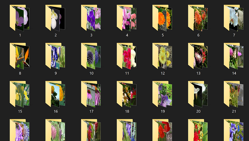

Each of the folders contains subfolders with a key identifier. Each of the folders contains flowers using the same key and is then evaluated to the flower's name using the JSON file.

{"21": "fire lily", "3": "canterbury bells", "45": "bolero deep blue", "1": "pink primrose", "34": "mexican aster", ......... }

One more thing we plan to do before feeding the images directly into the Datasets is augmenting the images to create more dynamic pictures to evaluate. PyTorch Uses the 'transforms.Compose' function to implement this. The code below is an example of creating augmentation of the image files.

normalize = transforms.Normalize(mean=[0.485, 0.456, 0.406],
                                 std=[0.229, 0.224, 0.225])

training_transforms = transforms.Compose([
    transforms.RandomResizedCrop(size=256, scale=(0.8, 1.0)),
    transforms.RandomRotation(15),
    transforms.ColorJitter(),
    transforms.RandomHorizontalFlip(),
    transforms.CenterCrop(size=224),
    transforms.ToTensor(),
    normalize
    ])

validation_transforms = transforms.Compose([
    transforms.Resize(256),
    transforms.CenterCrop(224),
    transforms.ToTensor(),
    normalize
    ])

testing_transforms = transforms.Compose([
    transforms.Resize(256),
    transforms.CenterCrop(224),
    transforms.ToTensor(),
    normalize
    ])

Let's now add the code to load these images into datasets in PyTorch to train the VGG models.

training_imagefolder = datasets.ImageFolder(train_dir, transform = training_transforms)
validation_imagefolder = datasets.ImageFolder(valid_dir, transform = validation_transforms)
testing_imagefolder = datasets.ImageFolder(test_dir, transform=testing_transforms)

train_loader = DataLoader(training_imagefolder,batch_size=tr_batchsize, shuffle=True)
validate_loader = DataLoader(validation_imagefolder, batch_size=eval_test_batchsize, shuffle=True)
test_loader = DataLoader(testing_imagefolder, batch_size=eval_test_batchsize, shuffle=True)

Training and Validating Models

def train_eval(model, traindataloader, validateloader, TrCriterion, optimizer, epochs, deviceFlag_train):
    model.to(deviceFlag_train)
    print(f'The training batchsize is {tr_batchsize}.')

    since = time.time() 
    for e in range(epochs): 
        itrs = 0
        model.train()

        for inputs, labels in tqdm(iter(traindataloader)):
            itrs += 1
            inputs = inputs.to(deviceFlag_train)
            labels = labels.to(deviceFlag_train)
            optimizer.zero_grad()
            outputs = model.forward(inputs)
            train_loss = TrCriterion(outputs, labels)
            train_loss.backward()
            optimizer.step()

        #Perform Validation
        with torch.no_grad():
            validation_loss, val_acc = validation(model, validateloader, TrCriterion)
   

        end = time.time()
        elapsed = end -since
        display = f' Epoch: {e + 1}/{epochs}, itrs:{itrs},'
        display += f' Valid_loss : {round(validation_loss, 4)},'
        display += f' Valid_Acc: {round(val_acc, 4)}' 
        display += f' Current time : {round(elapsed, 4)} sec'
        print(display)

Now we need to build the validation process to work through our validation tests set and give us an idea of how our model is doing.

def validation(model, validateloader, ValCriterion):
    model.eval()  # Set the model to evaluation mode
    val_loss_running = 0
    accuracy = 0
    
    with torch.no_grad():  # Turn off gradients for validation, saves memory and computations
        for images, labels in validateloader:
            images, labels = images.to(deviceFlag), labels.to(deviceFlag)
            output = model(images)
            val_loss_running += ValCriterion(output, labels).item()
            
            # Calculate accuracy
            ps = torch.exp(output)  # Convert log probabilities to probabilities
            top_p, top_class = ps.topk(1, dim=1)  # Get the indices of the top probability
            equals = top_class == labels.view(*top_class.shape)  # Reshape labels to match top_class dimensions
            accuracy += torch.mean(equals.type(torch.FloatTensor)).item()
            
    # Calculate average losses and accuracy
    val_loss = val_loss_running / len(validateloader)
    val_accuracy = accuracy / len(validateloader)
    
    model.train()  # Make sure to set model back to train mode
    return val_loss, val_accuracy

The last thing we need to do is save the model once it is produced. I've run the learning process without this step, let me tell you it's sad waiting for 30+ minutes to realize you aren't actually doing anything with your model and will have to run it all over again.

def save_checkpoint(model, optimizer, trainingdataset, saved_path):
    model.class_to_idx = trainingdataset.class_to_idx
    chkpt = {
            'arch': 'vgg19',
            'class_to_idx': model.class_to_idx,
            'model_state_dict': model.state_dict()
            }
    torch.save(chkpt, saved_path)

Building the Model

Perfect now we have all of the code in place to generate the training, we just have to sit back and "weight". (Yes it's a bad Neural Network pun..)

Found 1 GPU.

Now the device is set to cuda:0

The training batchsize is 32.

100%|███████████████████████████████████████████████████████████████████████████████████| 205/205 [00:55<00:00,  3.72it/s]

 Epoch: 1/10, itrs:205, Valid_loss : 1.0853, Valid_Acc: 0.7115 Current time : 64.3285 sec

100%|███████████████████████████████████████████████████████████████████████████████████| 205/205 [00:47<00:00,  4.35it/s]

 Epoch: 2/10, itrs:205, Valid_loss : 0.8346, Valid_Acc: 0.7736 Current time : 119.5268 sec

100%|███████████████████████████████████████████████████████████████████████████████████| 205/205 [00:48<00:00,  4.20it/s]

 Epoch: 3/10, itrs:205, Valid_loss : 0.8753, Valid_Acc: 0.7796 Current time : 176.9802 sec

100%|███████████████████████████████████████████████████████████████████████████████████| 205/205 [00:51<00:00,  3.97it/s]

 Epoch: 4/10, itrs:205, Valid_loss : 0.8736, Valid_Acc: 0.8085 Current time : 238.0622 sec

100%|███████████████████████████████████████████████████████████████████████████████████| 205/205 [00:56<00:00,  3.60it/s]

 Epoch: 5/10, itrs:205, Valid_loss : 0.87, Valid_Acc: 0.8253 Current time : 305.2062 sec

100%|███████████████████████████████████████████████████████████████████████████████████| 205/205 [00:58<00:00,  3.53it/s]

 Epoch: 6/10, itrs:205, Valid_loss : 0.9512, Valid_Acc: 0.7921 Current time : 374.4991 sec

100%|███████████████████████████████████████████████████████████████████████████████████| 205/205 [01:02<00:00,  3.30it/s]

 Epoch: 7/10, itrs:205, Valid_loss : 0.8648, Valid_Acc: 0.8137 Current time : 447.8964 sec

100%|███████████████████████████████████████████████████████████████████████████████████| 205/205 [01:05<00:00,  3.14it/s]

 Epoch: 8/10, itrs:205, Valid_loss : 0.8629, Valid_Acc: 0.8145 Current time : 525.3089 sec

100%|███████████████████████████████████████████████████████████████████████████████████| 205/205 [01:11<00:00,  2.88it/s]

 Epoch: 9/10, itrs:205, Valid_loss : 0.9773, Valid_Acc: 0.8073 Current time : 607.8328 sec

100%|███████████████████████████████████████████████████████████████████████████████████| 205/205 [01:11<00:00,  2.86it/s]

 Epoch: 10/10, itrs:205, Valid_loss : 1.0394, Valid_Acc: 0.7961 Current time : 691.568 sec

Test_acc : 79.61, time_spend: 11.01 sec

Now we are done and can give it a test!

Testing

The first thing we want to cover is loading in the checkpoint we have created. This way we don't have to generate the model each time we want to test out a new picture.

def load_checkpoint(chkpt_path):
    chkpt = torch.load(chkpt_path)
    model = models.vgg19(weights="DEFAULT")
    for params in model.parameters():
        params.requires_grad = False

    model.class_to_idx = chkpt['class_to_idx']
    classifier = nn.Sequential(OrderedDict([
        ('fc1', nn.Linear(25088, 4096)),
        ('relu', nn.ReLU()),
        ('drop', nn.Dropout(p=0.5)),
        ('fc2', nn.Linear(4096, 102)),
        ('output', nn.LogSoftmax(dim=1))
        ]))
    model.classifier = classifier
    model.to(deviceFlag)
    model.load_state_dict(chkpt['model_state_dict'])
    return model

We will then preprocess the image we want to test. We use these functions to do the heavy lifting.

def image_preprocessing(img_path):
    pil_image = Image.open(img_path)
    if pil_image.size[0] > pil_image.size[1]:
        pil_image.thumbnail((10000000, 256))
    else:
        pil_image.thumbnail((256, 10000000))

    #Crop
    left_margin = (pil_image.width - 244) / 2
    bottom_margin = (pil_image.height - 244) / 2
    right_margin = left_margin + 244
    top_margin = bottom_margin + 244

    pil_image = pil_image.crop((int(left_margin), int(bottom_margin), int(right_margin), int(top_margin)))

    #Convert to np then normalize
    np_image = np.array(pil_image) /255
    mean = np.array([0.485, 0.456, 0.406])
    std = np.array([0.229, 0.224, 0.225])
    np_image = (np_image - mean) /std

    np_image = np_image.transpose([2,0,1])
    return np_image

def imshow(pt_image, ax=None, title=None):
    if ax is None:
        fig, ax = plt.subplots()

    plt_image = pt_image.transpose((1,2,0))
    mean = np.array([0.485,0.456,0.406])
    std = np.array([0.229, 0.224, 0.225])
    plt_image = plt_image *std+mean

    if title is not None:
        ax.set_title(title)

    plt_image = np.clip(plt_image, 0, 1)
    ax.imshow(plt_image)
    return ax

def predict(img_path, model, trainingdataset, topk):
    np_img = image_preprocessing(img_path)
    pt_img = torch.from_numpy(np_img).float().to('cuda')
    pt_img = pt_img.unsqueeze(0)
    output = model.forward(pt_img)
    probs=torch.exp(output)
    top_probs, top_indices = probs.topk(topk)
    top_probs = top_probs.detach().to('cpu').numpy().tolist()[0]
    top_indices = top_indices.detach().to('cpu').numpy().tolist()[0]

    idx_to_class = {value: key for key, value in trainingdataset.class_to_idx.items()}
    top_classname = {idx_to_class[index] for index in top_indices}
    return top_probs, top_classname

Greate the last step is to call the functions above and to select the image we want to evaluate.

# Loads the created model
model = load_checkpoint('chkpt.pth')

probs, classes = predict('flowers/test/15/image_06369.jpg', model, training_imagefolder, 5)   
print(probs)
print(classes)

# Display an image along with the top 5 classes

# Plot flower input image
plt.figure(figsize = (6,10))
plot_1 = plt.subplot(2,1,1)

image = image_preprocessing('flowers/test/15/image_06369.jpg')

flower_title = flower_to_name['15']

imshow(image, plot_1, title=flower_title);

# Convert from the class integer encoding to actual flower names
flower_names = [flower_to_name[i] for i in classes]

# Plot the probabilities for the top 5 classes as a bar graph
plt.subplot(2,1,2)

sb.barplot(x=probs, y=flower_names, color=sb.color_palette()[0]);

plt.show()

This is what the window shows once it has been evaluated. Perfect it got it correct! The numbers below are the percentage of likelihood for each of the different flowers. The numbers below are the numbers of the flowers, which are parsed using the JSON in the dataset section above.

[0.9999998807907104, 9.838115744287279e-08, 1.4174122320298466e-08, 2.80199530244829e-09, 2.695716760925393e-09]
{'15', '46', '53', '90', '42'}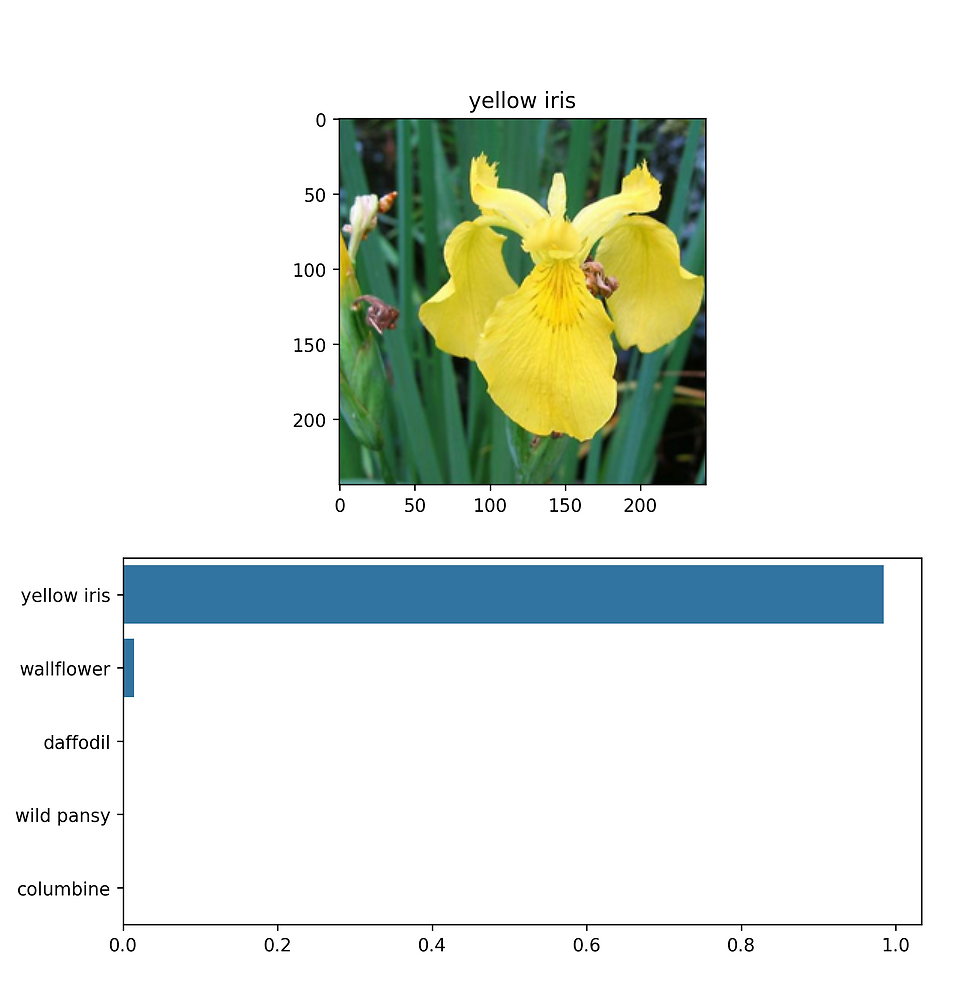

Conclusion

This is the first real run-through of the project. I am planning to add more metrics and models to the code to be compared and improved. Some of the tools we will be using will be a scheduler and Tensorboard. Stay tuned for future updates!